Supported Implementation#

Create OPE Input#

Before proceeding to OPE/OPS, we first create input_dict to enable a smooth implementation.

# create input for OPE class
from scope_rl.ope import CreateOPEInput
prep = CreateOPEInput(
    env=env,
)
input_dict = prep.obtain_whole_inputs(
    logged_dataset=logged_dataset,
    evaluation_policies=evaluation_policies,
    require_value_prediction=True,  # use model-based prediction
    n_trajectories_on_policy_evaluation=100,
    random_state=random_state,
)

Tip

See also

Supported Implementation (learning) describes how to obtain logged_dataset using a behavior policy in detail.

Basic Off-Policy Evaluation (OPE)#

The goal of (basic) OPE is to evaluate the following expected trajectory-wise reward of a policy (referred to as policy value).

\[J(\pi) := \mathbb{E}_{\tau} \left [ \sum_{t=0}^{T-1} \gamma^t r_{t} \mid \pi \right ],\]

where \(\pi\) is the (evaluation) policy, \(\tau\) is the trajectory observed by the evaluation policy, and \(r_t\) is the immediate reward at each timestep. (Please refer to the problem setup for additional notations.)

Here, we describe the class for conducting OPE and the implemented OPE estimators for estimating the policy value. We begin with the OffPolicyEvaluation class to streamline the OPE procedure.

# initialize the OPE class
from scope_rl.ope import OffPolicyEvaluation as OPE
ope = OPE(
    logged_dataset=logged_dataset,
    ope_estimators=[DM(), TIS(), PDIS(), DR()],
)

Using the OPE class, we can obtain the OPE results of various estimators at once as follows.

ope_dict = ope.estimate_policy_value(input_dict)

Tip

How to conduct OPE with multiple logged datasets?

Conducting OPE with multiple logged datasets requires no additional effort.

First, the same command with the single logged dataset case also works with multiple logged datasets.

ope = OPE(
    logged_dataset=logged_dataset,  # MultipleLoggedDataset
    ope_estimators=[DM(), TIS(), PDIS(), DR()],
)
multiple_ope_dict = ope.estimate_policy_value(
    input_dict,  # MultipleInputDict
)

The returned value is a dictionary containing the ope result.

In addition, we can specify which logged dataset and input_dict to use by setting behavior_policy_name and dataset_id.

multiple_ope_dict = ope.estimate_policy_value(
    input_dict,
    behavior_policy_name=behavior_policy.name,  #
    dataset_id=0,  # specify which logged dataset and input_dict to use
)

The basic visualization function also works by specifying the dataset id.

ope.visualize_off_policy_estimates(
    input_dict,
    behavior_policy_name=behavior_policy.name,
    dataset_id=0,  #
    ...,
)

policy value estimated with the specified dataset

Moreover, we provide additional visualization functions for the case with multiple logged datasets.

ope.visualize_policy_value_with_multiple_estimates(
    input_dict,      # MultipleInputDict
    behavior_policy_name=None,                   # compare estimators with multiple behavior policies
    # behavior_policy_name=behavior_policy.name  # compare estimators with a single behavior policy
    plot_type="ci",  # one of {"ci", "violin", "scatter"}, default="ci"
    ...,
)

When the plot_type is “ci”, the plot is somewhat similar to the basic visualization. (The star indicates the ground-truth policy value and the confidence intervals are derived by multiple estimates across datasets.)

policy value estimated with the multiple datasets

When the plot_type is “violin”, the plot visualizes the distribution of multiple estimates. This is particularly useful to see how the estimation result can vary depending on different datasets or random seeds.

policy value estimated with the multiple datasets (violin)

Finally, when the plot_type is “scatter”, the plot visualizes each estimation with its color specifying the behavior policy. This function is particularly useful to see how the choice of behavior policy (e.g., their stochasticity) affects the estimation result.

policy value estimated with the multiple datasets (scatter)

See also

Quickstart and related example codes

The OPE class implements the following functions.

(OPE)

estimate_policy_value
estimate_intervals
summarize_off_policy_estimates

(Evaluation of OPE estimators)

evaluate_performance_of_ope_estimators

(Visualization)

visualize_off_policy_estimates

(Visualization with multiple estimates on multiple logged datasets)

visualize_policy_value_with_multiple_estimates

Below, we describe the implemented OPE estimators.

Standard OPE estimators
Direct Method (DM)
Trajectory-wise Importance Sampling (TIS)
Per-Decision Importance Sampling (PDIS)
Doubly Robust (DR)
Self-Normalized estimators

Marginal OPE estimators
State Marginal estimators
State-Action Marginal estimators
Double Reinforcement Learning
Spectrum of Off-Policy Evaluation

Extensions
High Confidence Off-Policy Evaluation
Extension to the continuous action space

Tip

Direct Method (DM)#

DM [3] is a model-based approach that uses the initial state value (estimated by e.g., Fitted Q Evaluation (FQE) [4]). It first learns the Q-function and then leverages the learned Q-function as follows.

\[\hat{J}_{\mathrm{DM}} (\pi; \mathcal{D}) := \frac{1}{n} \sum_{i=1}^n \sum_{a \in \mathcal{A}} \pi(a | s_{0}^{(i)}) \hat{Q}(s_{0}^{(i)}, a) = \frac{1}{n} \sum_{i=1}^n \hat{V}(s_{0}^{(i)}),\]

where \(\mathcal{D}=\{\{(s_t, a_t, r_t)\}_{t=0}^{T-1}\}_{i=1}^n\) is the logged dataset with \(n\) trajectories. \(T\) indicates step per episode. \(\hat{Q}(s_t, a_t)\) is the estimated state-action value and \(\hat{V}(s_t)\) is the estimated state value.

DM has low variance compared to other estimators, but can produce larger bias due to approximation errors.

DirectMethod

Note

We use the implementation of FQE provided by d3rlpy.

Trajectory-wise Importance Sampling (TIS)#

TIS [5] uses the importance sampling technique to correct the distribution shift between \(\pi\) and \(\pi_0\) as follows.

\[\hat{J}_{\mathrm{TIS}} (\pi; \mathcal{D}) := \frac{1}{n} \sum_{i=1}^n \sum_{t=0}^{T-1} \gamma^t w_{1:T-1}^{(i)} r_t^{(i)},\]

where \(w_{0:T-1} := \prod_{t=0}^{T-1} (\pi(a_t | s_t) / \pi_0(a_t | s_t))\) is the trajectory-wise importance weight.

TIS enables an unbiased estimation of the policy value. However, when the trajectory length \(T\) is large, TIS suffers from high variance due to the product of importance weights over the entire horizon.

TrajectoryWiseImportanceSampling

Per-Decision Importance Sampling (PDIS)#

PDIS [5] leverages the sequential nature of the MDP to reduce the variance of TIS. Specifically, since \(s_t\) only depends on \(s_0, \ldots, s_{t-1}\) and \(a_0, \ldots, a_{t-1}\) and is independent of \(s_{t+1}, \ldots, s_{T}\) and \(a_{t+1}, \ldots, a_{T}\), PDIS only considers the importance weight of the past interactions when estimating \(r_t\) as follows.

\[\hat{J}_{\mathrm{PDIS}} (\pi; \mathcal{D}) := \frac{1}{n} \sum_{i=1}^n \sum_{t=0}^{T-1} \gamma^t w_{0:t}^{(i)} r_t^{(i)},\]

where \(w_{0:t} := \prod_{t'=0}^t (\pi(a_{t'} | s_{t'}) / \pi_b(a_{t'} | s_{t'}))\) is the importance weight for each time step wrt the previous actions.

PDIS remains unbiased while reducing the variance of TIS. However, when \(t\) is large, PDIS still suffers from high variance.

PerDecisionImportanceSampling

Doubly Robust (DR)#

DR [6, 7] is a hybrid of model-based estimation and importance sampling. It introduces \(\hat{Q}\) as a baseline estimation in the recursive form of PDIS and applies importance weighting only on its residual.

\[\hat{J}_{\mathrm{DR}} (\pi; \mathcal{D}) := \frac{1}{n} \sum_{i=1}^n \sum_{t=0}^{T-1} \gamma^t \left(w_{0:t}^{(i)} (r_t^{(i)} - \hat{Q}(s_t^{(i)}, a_t^{(i)})) + w_{0:t-1}^{(i)} \sum_{a \in \mathcal{A}} \pi(a | s_t^{(i)}) \hat{Q}(s_t^{(i)}, a) \right),\]

DR is unbiased and has lower variance than PDIS when \(\hat{Q}(\cdot)\) is reasonably accurate to satisfy \(0 < \hat{Q}(\cdot) < 2 Q(\cdot)\). However, when the importance weight is quite large, it may still suffer from high variance.

DoublyRobust

Self-Normalized estimators#

Self-normalized estimators [11] aim to reduce the scale of importance weight for the variance reduction purpose. Specifically, the self-normalized versions of PDIS and DR are defined as follows.

\[\hat{J}_{\mathrm{SNPDIS}} (\pi; \mathcal{D}) := \sum_{i=1}^n \sum_{t=0}^{T-1} \gamma^t \frac{w_{0:t}^{(i)}}{\sum_{i'=1}^n w_{0:t}^{(i')}} r_t^{(i)},\]

\[\hat{J}_{\mathrm{SNDR}} (\pi; \mathcal{D}) := \sum_{i=1}^n \sum_{t=0}^{T-1} \gamma^t \left(\frac{w_{0:t}^{(i)}}{\sum_{i'=1}^n w_{0:t}^{(i')}} (r_t^{(i)} - \hat{Q}(s_t^{(i)}, a_t^{(i)})) + \frac{w_{0:t-1}^{(i)}}{\sum_{i'=1}^n w_{0:t-1}^{(i')}} \sum_{a \in \mathcal{A}} \pi(a | s_t^{(i)}) \hat{Q}(s_t^{(i)}, a) \right),\]

In more general, self-normalized estimators substitute the importance weight \(w_{\ast}\) as follows.

\[\tilde{w}_{\ast} := \frac{w_{\ast}}{\sum_{i=1}^n w_{\ast}}\]

where \(\tilde{w}_{\ast}\) is the self-normalized importance weight.

Self-normalized estimators are no longer unbiased, but have variance bounded by \(r_{max}^2\) while also remaining consistent.

SelfNormalizedTIS

SelfNormalizedPDIS

SelfNormalizedDR

Marginalized Importance Sampling Estimators#

When the length of the trajectory (\(T\)) is large, even per-decision importance weights can be exponentially large in the latter part of the trajectory. To alleviate this, state marginal or state-action marginal importance weights can be used instead of the per-decision importance weight as follows [12, 13].

\[\begin{split}\rho(s, a) &:= d^{\pi}(s, a) / d^{\pi_0}(s, a) \\ \rho(s) &:= d^{\pi}(s) / d^{\pi_0}(s)\end{split}\]

\(d^{\pi}(s, a)\) and \(d^{\pi}(s)\) is the marginal visitation probability of the policy \(\pi\) on \((s, a)\) or \(s\), respectively. The use of marginal importance weights is particularly beneficial when policy visits the same or similar states among different trajectories or different timesteps. (e.g., when the state transition is something like \(\cdots \rightarrow s_1 \rightarrow s_2 \rightarrow s_1 \rightarrow s_2 \rightarrow \cdots\) or when the trajectories always visits some particular state as \(\cdots \rightarrow s_{*} \rightarrow s_{1} \rightarrow s_{*} \rightarrow \cdots\)). Then, State-Action Marginal Importance Sampling (SMIS) and State Marginal Doubly Robust (SMDR) are defined as follows.

\[\hat{J}_{\mathrm{SAM-IS}} (\pi; \mathcal{D}) := \frac{1}{n} \sum_{i=1}^n \sum_{t=0}^{T-1} \gamma^t \rho(s_t^{(i)}, a_t^{(i)}) r_t^{(i)},\]

\[\begin{split}\hat{J}_{\mathrm{SAM-DR}} (\pi; \mathcal{D}) &:= \frac{1}{n} \sum_{i=1}^n \sum_{a \in \mathcal{A}} \pi(a | s_0^{(i)}) \hat{Q}(s_0^{(i)}, a) \\ & \quad \quad + \frac{1}{n} \sum_{i=1}^n \sum_{t=0}^{T-1} \gamma^t \rho(s_t^{(i)}, a_t^{(i)}) \left(r_t^{(i)} + \gamma \sum_{a \in \mathcal{A}} \pi(a | s_t^{(i)}) \hat{Q}(s_{t+1}^{(i)}, a) - \hat{Q}(s_t^{(i)}, a_t^{(i)}) \right),\end{split}\]

Similarly, State-Marginal Importance Sampling (SAMIS) and State Action-Marginal Doubly Robust (SAMDR) are defined as follows.

\[\hat{J}_{\mathrm{SM-IS}} (\pi; \mathcal{D}) := \frac{1}{n} \sum_{i=1}^n \sum_{t=0}^{T-1} \gamma^t \rho(s_t^{(i)}) w_t(s_t^{(i)}, a_t^{(i)}) r_t^{(i)},\]

\[\begin{split}\hat{J}_{\mathrm{SM-DR}} (\pi; \mathcal{D}) &:= \frac{1}{n} \sum_{i=1}^n \sum_{a \in \mathcal{A}} \pi(a | s_0^{(i)}) \hat{Q}(s_0^{(i)}, a) \\ & \quad \quad + \frac{1}{n} \sum_{i=1}^n \sum_{t=0}^{T-1} \gamma^t \rho(s_t^{(i)}) w_t(s_t^{(i)}, a_t^{(i)}) \left(r_t^{(i)} + \gamma \sum_{a \in \mathcal{A}} \pi(a | s_t^{(i)}) \hat{Q}(s_{t+1}^{(i)}, a) - \hat{Q}(s_t^{(i)}, a_t^{(i)}) \right),\end{split}\]

where \(w_t(s_t, a_t) := \pi(a_t | s_t) / \pi_0(a_t | s_t)\) is the immediate importance weight at timestep \(t\).

Tip

We implement state marginal and state-action marginal OPE estimators in the following classes (both for Discrete- and Continuous- action spaces).

(State Marginal Estimators)

StateMarginalDM

StateMarginalIS

StateMarginalDR

StateMarginalSNIS

StateMarginalSNDR

(State-Action Marginal Estimators)

StateActionMarginalIS

StateActionMarginalDR

StateActionMarginalSNIS

StateActionMarginalSNDR

Double Reinforcement Learning (DRL)#

Comparing DR in the standard and marginal OPE, we notice that their formulation is slightly different as follows.

(DR in standard OPE)

\[\hat{J}_{\mathrm{DR}} (\pi; \mathcal{D}) := \frac{1}{n} \sum_{i=1}^n \sum_{t=0}^{T-1} \gamma^t \left( w_{0:t}^{(i)} (r_t^{(i)} - \hat{Q}(s_t^{(i)}, a_t^{(i)})) + w_{0:t-1}^{(i)} \sum_{a \in \mathcal{A}} \pi(a | s_t^{(i)}) \hat{Q}(s_t^{(i)}, a) \right),\]

(DR in marginal OPE)

Then, a natural question arises, would it be possible to use marginal importance weight in DR in the standard formulation?

DRL [15] leverages the marginal importance sampling in the standard OPE formulation as follows.

\[\begin{split}\hat{J}_{\mathrm{DRL}} (\pi; \mathcal{D}) & := \frac{1}{n} \sum_{k=1}^K \sum_{i=1}^{n_k} \sum_{t=0}^{T-1} (\rho^j(s_{t}^{(i)}, a_{t}^{(i)}) (r_{t}^{(i)} - Q^j(s_{t}^{(i)}, a_{t}^{(i)})) \\ & \quad \quad + \rho^j(s_{t-1}^{(i)}, a_{t-1}^{(i)}) \sum_{a \in \mathcal{A}} \pi(a | s_t^{(i)}) Q^j(s_{t}^{(i)}, a))\end{split}\]

DRL achieves the semiparametric efficiency bound with a consistent value predictor \(Q\). Therefore, to alleviate the potential bias introduced in \(Q\), DRL uses the “cross-fitting” technique to estimate the value function. Specifically, let \(K\) is the number of folds and \(\mathcal{D}_j\) is the \(j\)-th split of logged data consisting of \(n_k\) samples. Cross-fitting trains \(\rho^j\) and \(Q^j\) on the subset of data used for OPE, i.e., \(\mathcal{D} \setminus \mathcal{D}_j\).

DoubleReinforcementLearning

Tip

Spectrum of Off-Policy Estimators (SOPE)#

While state marginal or state-action marginal importance weight effectively alleviates the variance of per-decision importance weight, the estimation error of marginal importance weights may introduce some bias in estimation. To alleviate this and control the bias-variance tradeoff more flexibly, SOPE uses the following interpolated importance weights [14].

\[\begin{split}w_{\mathrm{SOPE}}(s_t, a_t) &= \begin{cases} \prod_{t'=0}^{k-1} w_t(s_{t'}, a_{t'}) & \mathrm{if} \, t < k \\ \rho(s_{t-k}, a_{t-k}) \prod_{t'=t-k+1}^{t} w_t(s_{t'}, a_{t'}) & \mathrm{otherwise} \end{cases} \\ w_{\mathrm{SOPE}}(s_t, a_t) &= \begin{cases} \prod_{t'=0}^{k-1} w_t(s_{t'}, a_{t'}) & \mathrm{if} \, t < k \\ \rho(s_{t-k}) \prod_{t'=t-k}^{t} w_t(s_{t'}, a_{t'}) & \mathrm{otherwise} \end{cases}\end{split}\]

where SOPE uses per-decision importance weight \(w_t(s_t, a_t) := \pi(a_t | s_t) / \pi_0(a_t | s_t)\) for the \(k\) most recent timesteps.

For instance, State Action-Marginal Importance Sampling (SAMIS) and State Action-Marginal Doubly Robust (SAM-DR) are defined as follows.

\[\hat{J}_{\mathrm{SOPE-SAM-IS}} (\pi; \mathcal{D}) := \frac{1}{n} \sum_{i=1}^n \sum_{t=0}^{k-1} \gamma^t w_{0:t}^{(i)} r_t^{(i)} + \frac{1}{n} \sum_{i=1}^n \sum_{t=k}^{T-1} \gamma^t \rho(s_{t-k}^{(i)}, a_{t-k}^{(i)}) w_{t-k+1:t}^{(i)} r_t^{(i)},\]

\[\begin{split}\hat{J}_{\mathrm{SOPE-SAM-DR}} (\pi; \mathcal{D}) &:= \frac{1}{n} \sum_{i=1}^n \sum_{a \in \mathcal{A}} \pi(a | s_0^{(i)}) \hat{Q}(s_0^{(i)}, a) \\ & \quad \quad + \frac{1}{n} \sum_{i=1}^n \sum_{t=0}^{k-1} \gamma^t w_{0:t}^{(i)} \left(r_t^{(i)} + \gamma \sum_{a \in \mathcal{A}} \pi(a | s_t^{(i)}) \hat{Q}(s_{t+1}^{(i)}, a) - \hat{Q}(s_t^{(i)}, a_t^{(i)}) \right) \\ & \quad \quad + \frac{1}{n} \sum_{i=1}^n \sum_{t=k}^{T-1} \gamma^t \rho(s_{t-k}^{(i)}, a_{t-k}^{(i)}) w_{t-k+1:t}^{(i)} \left(r_t^{(i)} + \gamma \sum_{a \in \mathcal{A}} \pi(a | s_t^{(i)}) \hat{Q}(s_{t+1}^{(i)}, a) - \hat{Q}(s_t^{(i)}, a_t^{(i)}) \right),\end{split}\]

Tip

High Confidence Off-Policy Evaluation (HCOPE)#

To alleviate the risk of optimistically overestimating the policy value, we are sometimes interested in the confidence intervals and the lower bound of the estimated policy value. We implement four methods to estimate the confidence intervals [21, 22, 23].

Hoeffding [23]:

\[|\hat{J}(\pi; \mathcal{D}) - \mathbb{E}_{\mathcal{D}}[\hat{J}(\pi; \mathcal{D})]| \leq \hat{J}_{\max} \displaystyle \sqrt{\frac{\log(1 / \alpha)}{2 n}}.\]

Empirical Bernstein [21, 23]:

\[|\hat{J}(\pi; \mathcal{D}) - \mathbb{E}_{\mathcal{D}}[\hat{J}(\pi; \mathcal{D})]| \leq \displaystyle \frac{7 \hat{J}_{\max} \log(2 / \alpha)}{3 (n - 1)} + \displaystyle \sqrt{\frac{2 \hat{\mathbb{V}}_{\mathcal{D}}(\hat{J}) \log(2 / \alpha)}{(n - 1)}}.\]

Student T-test [21]:

\[|\hat{J}(\pi; \mathcal{D}) - \mathbb{E}_{\mathcal{D}}[\hat{J}(\pi; \mathcal{D})]| \leq \displaystyle \frac{T_{\mathrm{test}}(1 - \alpha, n-1)}{\sqrt{n} / \hat{\sigma}}.\]

Bootstrapping [21, 22]:

\[|\hat{J}(\pi; \mathcal{D}) - \mathbb{E}_{\mathcal{D}}[\hat{J}(\pi; \mathcal{D})]| \leq \mathrm{Bootstrap}(1 - \alpha).\]

Note that all the above bound holds with probability \(1 - \alpha\). For notations, we denote \(\hat{\mathbb{V}}_{\mathcal{D}}(\cdot)\) to be the sample variance, \(T_{\mathrm{test}}(\cdot,\cdot)\) to be T value, and \(\sigma\) to be the standard deviation.

Among the above high confidence interval estimation, hoeffding and empirical bernstein derives a lower bound without any distribution assumption of \(p(\hat{J})\), which sometimes leads to quite conservative estimation. On the other hand, T-test is based on the assumption that each sample of \(p(\hat{J})\) follows the normal distribution.

Tip

Extension to the Continuous Action Space#

When the action space is continuous, the naive importance weight \(w_t = \pi(a_t|s_t) / \pi_0(a_t|s_t) = (\pi(a |s_t) / \pi_0(a_t|s_t)) \cdot \mathbb{I} \{a = a_t \}\) rejects almost every actions, as the indicator function \(\mathbb{I}\{a = a_t\}\) filters only the action observed in the logged data.

To address this issue, continuous-action OPE estimators apply kernel density estimation technique to smooth the importance weight [57, 58].

\[\overline{w}_t = \int_{a \in \mathcal{A}} \frac{\pi(a | s_t)}{\pi_0(a_t | s_t)} \cdot \frac{1}{h} K \left( \frac{a - a_t}{h} \right) da,\]

where \(K(\cdot)\) denotes a kernel function and \(h\) is the bandwidth hyperparameter. We can use any function as \(K(\cdot)\) that meets the following qualities:

1. \(\int xK(x) dx = 0\),
1. \(\int K(x) dx = 1\),
1. \(\lim _{x \rightarrow-\infty} K(x)=\lim _{x \rightarrow+\infty} K(x)=0\),
1. \(K(x) \geq 0, \forall x\).

We provide the following kernel functions in SCOPE-RL.

Gaussian kernel: \(K(x) = \frac{1}{\sqrt{2 \pi}} e^{-\frac{x^{2}}{2}}\)
Epanechnikov kernel: \(K(x) = \frac{3}{4} (1 - x^2) \, (|x| \leq 1)\)
Triangular kernel: \(K(x) = 1 - |x| \, (|x| \leq 1)\)
Cosine kernel: \(K(x) = \frac{\pi}{4} \mathrm{cos} \left( \frac{\pi}{2} x \right) \, (|x| \leq 1)\)
Uniform kernel: \(K(x) = \frac{1}{2} \, (|x| \leq 1)\)

Tip

Cumulative Distribution Off-Policy Evaluation (CD-OPE)#

While the basic OPE aims to estimate the average policy performance, we are often also interested in the performance distribution of the evaluation policy. Cumulative distribution OPE enables flexible estimation of various risk functions such as variance and conditional value at risk (CVaR) using the cumulative distribution function (CDF) [8, 9, 10].

(Cumulative Distribution Function)

\[F(m, \pi) := \mathbb{E} \left[ \mathbb{I} \left \{ \sum_{t=0}^{T-1} \gamma^t r_t \leq m \right \} \mid \pi \right]\]

(Risk Functions derived by CDF)

Mean: \(\mu(F) := \int_{G} G \, \mathrm{d}F(G)\)
Variance: \(\sigma^2(F) := \int_{G} (G - \mu(F))^2 \, \mathrm{d}F(G)\)
\(\alpha\)-quartile: \(Q^{\alpha}(F) := \min \{ G \mid F(G) \leq \alpha \}\)
Conditional Value at Risk (CVaR): \(\int_{G} G \, \mathbb{I}\{ G \leq Q^{\alpha}(F) \} \, \mathrm{d}F(G)\)

where we let \(G := \sum_{t=0}^{T-1} \gamma^t r_t\) to represent the trajectory-wise reward as a random variable and \(dF(G) := \mathrm{lim}_{\Delta \rightarrow 0} F(G) - F(G- \Delta)\).

To estimate both CDF and various risk functions, we provide the following CumulativeDistributionOffPolicyEvaluation class.

# initialize the OPE class
from scope_rl.ope import CumulativeDistributionOPE
cd_ope = CumulativeDistributionOPE(
    logged_dataset=logged_dataset,
    ope_estimators=[CD_DM(), CD_IS(), CD_DR()],
)

It estimates the cumulative distribution of the trajectory-wise reward and various risk functions as follows.

cdf_dict = cd_ope.estimate_cumulative_distribution_function(input_dict)
variance_dict = cd_ope.estimate_variance(input_dict)

Tip

How to conduct Cumulative Distribution OPE with multiple logged datasets?

Conducting Cumulative Distribution OPE with multiple logged datasets requires no additional efforts.

First, the same command with the single logged dataset case also works with multiple logged datasets.

ope = CumulativeDistributionOPE(
    logged_dataset=logged_dataset,  # MultipleLoggedDataset
    ope_estimators=[CD_DM(), CD_IS(), CD_DR()],
)
multiple_cdf_dict = ope.estimate_cumulative_distribution_function(
    input_dict,  # MultipleInputDict
)

The returned value is the dictionary containing the ope result.

In addition, we can specify which logged dataset and input_dict to use by setting behavior_policy_name and dataset_id.

multiple_ope_dict = ope.estimate_cumulative_distribution_function(
    input_dict,
    behavior_policy_name=behavior_policy.name,  #
    dataset_id=0,  # specify which logged dataset and input_dict to use
)

The basic visualization function also works by specifying the dataset id.

ope.visualize_cumulative_distribution_function(
    input_dict,
    behavior_policy_name=behavior_policy.name,  #
    dataset_id=0,  #
    random_state=random_state,
)

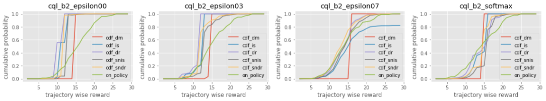
cumulative distribution function estimated with the specified dataset

Moreover, we provide additional visualization functions for the multiple logged dataset case.

The following visualizes confidence intervals of the cumulative distribution function.

ope.visualize_cumulative_distribution_function_with_multiple_estimates(
    input_dict,      # MultipleInputDict
    behavior_policy_name=None,                   # compare estimators with multiple behavior policies
    # behavior_policy_name=behavior_policy.name  # compare estimators with a single behavior policy
    random_state=random_state,
)

cumulative distribution function estimated with the multiple datasets

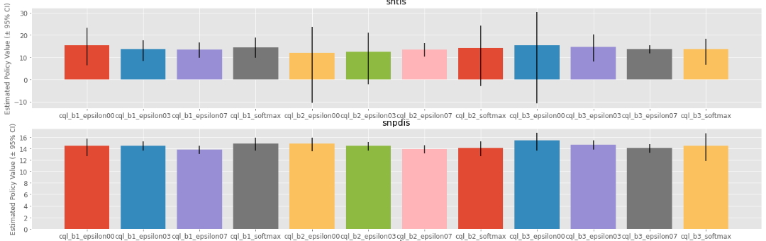
In contrast, the following visualizes the distribution of multiple estimates of point-wise policy performance (e.g., policy value, variance, conditional value at risk, lower quartile).

ope.visualize_policy_value_with_multiple_estimates(
    input_dict,      # MultipleInputDict
    plot_type="ci",  # one of {"ci", "violin", "scatter"}, default="ci"
    random_state=random_state,
)

policy value estimated with the multiple datasets

policy value estimated with the multiple datasets (violin)

policy value estimated with the multiple datasets (scatter)

See also

Quickstart and related example codes

CumulativeDistributionOffPolicyEvaluation implements the following functions.

(Cumulative Distribution Function)

estimate_cumulative_distribution_function

(Risk Functions and Statistics)

estimate_mean
estimate_variance
estimate_conditional_value_at_risk
estimate_interquartile_range

(Visualization)

visualize_policy_value
visualize_conditional_value_at_risk
visualize_interquartile_range
visualize_cumulative_distribution_function

(Visualization with multiple estimates on multiple logged datasets)

visualize_policy_value_with_multiple_estimates
visualize_variance_with_multiple_estimates
visualize_cumulative_distribution_function_with_multiple_estimates
visualize_lower_quartile_with_multiple_estimates
visualize_cumulative_distribution_function_with_multiple_estimates

(Others)

obtain_reward_scale

Below, we describe the implemented cumulative distribution OPE estimators.

Direct Method (DM)
Trajectory-wise Importance Sampling (TIS)
Trajectory-wise Doubly Robust (DR)
Self-Normalized estimators
Extension to the continuous action space

Tip

Direct Method (DM)#

DM adopts a model-based approach to estimate the cumulative distribution function.

\[\hat{F}_{\mathrm{DM}}(m, \pi; \mathcal{D}) := \frac{1}{n} \sum_{i=1}^n \sum_{a \in \mathcal{A}} \pi(a | s_0^{(i)}) \hat{G}(m; s_0^{(i)}, a)\]

where \(\hat{F}(\cdot)\) is the estimated cumulative distribution function and \(\hat{G}(\cdot)\) is an estimator for \(\mathbb{E} \left[ \mathbb{I} \left \{\sum_{t=0}^{T-1} \gamma^t r_t \leq m \right \} \mid s,a \right]\).

DM is vulnerable to the approximation error, but has low variance.

CumulativeDistributionDM

Trajectory-wise Importance Sampling (TIS)#

TIS corrects the distribution shift by applying the importance sampling technique on the cumulative distribution estimation.

\[\hat{F}_{\mathrm{TIS}}(m, \pi; \mathcal{D}) := \frac{1}{n} \sum_{i=1}^n w_{0:T-1}^{(i)} \mathbb{I} \left \{\sum_{t=0}^{T-1} \gamma^t r_t^{(i)} \leq m \right \}\]

where \(w_{0:T-1} := \prod_{t=0}^{T-1} (\pi(a_t | s_t) / \pi_0(a_t | s_t))\) is the trajectory-wise importance weight. TIS is unbiased but can suffer from high variance. As a consequence, \(\hat{F}_{\mathrm{TIS}}(\cdot)\) sometimes becomes more than 1.0 when the variance is high. Therefore, we correct CDF as follows [8].

\[\hat{F}^{\ast}_{\mathrm{TIS}}(m, \pi; \mathcal{D}) := \min(\max_{m' \leq m} \hat{F}_{\mathrm{TIS}}(m', \pi; \mathcal{D}), 1)\]

CumulativeDistributionTIS

Trajectory-wise Doubly Robust (TDR)#

TDR combines TIS and DM to reduce the variance while being unbiased.

\[\hat{F}_{\mathrm{TDR}}(m, \pi; \mathcal{D}) := \frac{1}{n} \sum_{i=1}^n w_{0:T-1}^{(i)} \left( \mathbb{I} \left \{\sum_{t=0}^{T-1} \gamma^t r_t^{(i)} \leq m \right \} - \hat{G}(m; s_0^{(i)}, a_0^{(i)}) \right) + \hat{F}_{\mathrm{DM}}(m, \pi; \mathcal{D})\]

TDR reduces the variance of TIS while being unbiased, leveraging the model-based estimate (i.e., DM) as a control variate. Since \(\hat{F}_{\mathrm{TDR}}(\cdot)\) may be less than zero or more than one, we should apply the following transformation to bound \(\hat{F}_{\mathrm{TDR}}(\cdot) \in [0, 1]\) [8].

\[\hat{F}^{\ast}_{\mathrm{TDR}}(m, \pi; \mathcal{D}) := \mathrm{clip}(\max_{m' \leq m} \hat{F}_{\mathrm{TDR}}(m', \pi; \mathcal{D}), 0, 1).\]

Note that this estimator is not equivalent to the (recursive) DR estimator defined by [9]. We are planning to implement the recursive version in a future update of the software.

CumulativeDistributionTDR

Finally, we also provide the self-normalized estimators for TIS and TDR. They use the self-normalized importance weight \(\tilde{w}_{\ast} := w_{\ast} / (\sum_{i=1}^{n} w_{\ast})\) for the variance reduction purpose.

CumulativeDistributionSNTIS

CumulativeDistributionSNDR

Evaluation Metrics of OPE/OPS#

Finally, we describe the metrics to evaluate the quality of OPE estimators and its OPS results.

Mean Squared Error (MSE) [24, 25, 26]:
This metric measures the estimation accuracy as \(\sum_{\pi \in \Pi} (\hat{J}(\pi; \mathcal{D}) - J(\pi))^2 / |\Pi|\).
Regret@k [24, 26]:
This metric measures how well the selected policy(ies) performs. In particular, Regret@1 indicates the expected performance difference between the (oracle) best policy and the selected policy as \(J(\pi^{\ast}) - J(\hat{\pi}^{\ast})\), where \(\pi^{\ast} := {\arg\max}_{\pi \in \Pi} J(\pi)\) and \(\hat{\pi}^{\ast} := {\arg\max}_{\pi \in \Pi} \hat{J}(\pi; \mathcal{D})\).
Spearman’s Rank Correlation Coefficient [24, 26]:
This metric measures how well the ranking of the candidate estimators is preserved in the OPE result.
Type I and Type II Error Rate:
This metric measures how well an OPE estimator validates whether the policy performance surpasses the given safety threshold or not.

To ease the comparison of candidate (evaluation) policies and the OPE estimators, we provide the OffPolicySelection class.

# Initialize the OPS class
from scope_rl.ope import OffPolicySelection
ops = OffPolicySelection(
    ope=ope,
    cumulative_distribution_ope=cd_ope,
)

The OffPolicySelection class returns both the OPE results and the OPS metrics as follows.

ranking_df, metric_df = ops.select_by_policy_value(
    input_dict,
    return_metrics=True,
    return_by_dataframe=True,
)

Moreover, the OPS class enables us to validate the best/worst/mean/std performance of top k deployment and how well the safety requirement is satisfied. Note that, we provide the detailed description of these top- \(k\) metrics and the proposed SharpeRatio@k metric in this page: Risk-Return Assessments of OPE via SharpeRatio@k.

ops.visualize_topk_policy_value_selected_by_standard_ope(
    input_dict=input_dict,
    safety_criteria=1.0,
)

Finally, the OPS class also implements the modules to compare the OPE result and the true policy metric as follows.

ops.visualize_policy_value_for_validation(
    input_dict=input_dict,
    n_cols=4,
    share_axes=True,
)

Tip

See also

Quickstart and related example codes

The OPS class implements the following functions.

(OPS)

obtain_oracle_selection_result
select_by_policy_value
select_by_policy_value_via_cumulative_distribution_ope
select_by_policy_value_lower_bound
select_by_lower_quartile
select_by_conditional_value_at_risk

(Visualization)

visualize_policy_value_for_selection
visualize_cumulative_distribution_function_for_selection
visualize_policy_value_for_selection
visualize_policy_value_of_cumulative_distribution_ope_for_selection
visualize_conditional_value_at_risk_for_selection
visualize_interquartile_range_for_selection

(Visualization with multiple estimates on multiple logged datasets)

visualize_policy_value_with_multiple_estimates_standard_ope
visualize_policy_value_with_multiple_estimates_cumulative_distribution_ope
visualize_variance_with_multiple_estimates
visualize_cumulative_distribution_function_with_multiple_estimates
visualize_lower_quartile_with_multiple_estimates
visualize_cumulative_distribution_function_with_multiple_estimates

(Visualization of top k performance)

visualize_topk_policy_value_selected_by_standard_ope
visualize_topk_policy_value_selected_by_cumulative_distribution_ope
visualize_topk_policy_value_selected_by_lower_bound
visualize_topk_conditional_value_at_risk_selected_by_standard_ope
visualize_topk_conditional_value_at_risk_selected_by_cumulative_distribution_ope
visualize_topk_lower_quartile_selected_by_standard_ope
visualize_topk_lower_quartile_selected_by_cumulative_distribution_ope

(Visualization for validation)

visualize_policy_value_for_validation
visualize_policy_value_of_cumulative_distribution_ope_for_validation
visualize_policy_value_lower_bound_for_validation
visualize_variance_for_validation
visualize_lower_quartile_for_validation
visualize_conditional_value_at_risk_for_validation

<<< Prev Problem Formulation

<<< Prev Offline RL

Next >>> Visualization tools

Next >>> Package Reference