Quickstart#
We show an example workflow of synthetic dataset collection, offline Reinforcement Learning (RL), to Off-Policy Evaluation (OPE). The workflow mainly consists of the following three steps (and a validation step):

Workflow of offline RL and OPE streamlined by SCOPE-RL
- Synthetic Dataset Generation and Data Preprocessing:
The initial step is to collect logged data using a behavior policy. In a synthetic setup, we first train a behavior policy through online interaction and then generate dataset(s) with the behavior policy. In a practical situation, we should use the preprocessed logged data obtained from real-world applications.
- Offline Reinforcement Learning:
We then learn new policies (, which hopefully perform better than the behavior policy) from only offline logged data, without any online interactions.
- Off-Policy Evaluation and Selection:
After learning several candidate policies offline, we need to choose the production policy. We consider a typical workflow that starts from screening out promising candidate policies through Off-Policy Evaluation (OPE) and then choosing the final production policy among the selected candidates based on more reliable online A/B tests result, as illustrated in the following figure.

Practical workflow of policy evaluation and selection
See also
Why SCOPE-RL? describes the distinctive features of SCOPE-RL in detail.
Overview (online/offline RL) and Overview (OPE/OPS) describe the problem settings.
Synthetic Dataset Generation and Data Preprocessing#
We start by collecting the logged data using DDQN [1] as a behavior policy. Note that in the following example, we use RTBGym (a sub-package of SCOPE-RL) and d3rlpy. Please satisfy the requirements in advance.
# implement data collection procedure on the RTBGym environment

# import SCOPE-RL modules
from scope_rl.dataset import SyntheticDataset
from scope_rl.policy import EpsilonGreedyHead
# import d3rlpy algorithms
from d3rlpy.algos import DoubleDQNConfig
from d3rlpy.dataset import create_fifo_replay_buffer
from d3rlpy.algos import ConstantEpsilonGreedy
# import rtbgym and gym
import rtbgym
import gym
import torch
# random state
random_state = 12345
device = "cuda:0" if torch.cuda.is_available() else "cpu"

# (0) Setup environment
env = gym.make("RTBEnv-discrete-v0")

# (1) Learn a baseline online policy (using d3rlpy)
# initialize the algorithm
ddqn = DoubleDQNConfig().create(device=device)
# train an online policy
ddqn.fit_online(
    env,
    buffer=create_fifo_replay_buffer(limit=10000, env=env),
    explorer=ConstantEpsilonGreedy(epsilon=0.3),
    n_steps=100000,
    n_steps_per_epoch=1000,
    update_start_step=1000,
)

# (2) Generate logged dataset
# convert ddqn policy into a stochastic behavior policy
behavior_policy = EpsilonGreedyHead(
    ddqn,
    n_actions=env.action_space.n,
    epsilon=0.3,
    name="ddqn_epsilon_0.3",
    random_state=random_state,
)
# initialize the dataset class
dataset = SyntheticDataset(
    env=env,
    max_episode_steps=env.step_per_episode,
)
# collect logged data by a behavior policy
train_logged_dataset = dataset.obtain_episodes(
    behavior_policies=behavior_policy,
    n_trajectories=10000,
    random_state=random_state,
)
test_logged_dataset = dataset.obtain_episodes(
    behavior_policies=behavior_policy,
    n_trajectories=10000,
    random_state= + 1,
)
Users can collect logged data from any environment with OpenAI Gym and Gymnasium-like interface using a variety of behavior policies. Moreover, by preprocessing the logged data, one can also handle their own logged data from real-world applications.
See also
Example codes and guidelines for using multiple logged datasets and real-world datasets
API references of dataset modules and policy wrapper (Head)
Offline Reinforcement Learning#
Now we are ready to learn a new policy only from logged data. Specifically, we learn a CQL [2] policy here. (Please also refer to Offline Reinforcement Learning about the problem setting and the algorithms.) Note that, we use d3rlpy for offline RL.
# implement offline RL procedure using scope_rl and d3rlpy

# import d3rlpy algorithms
from d3rlpy.dataset import MDPDataset
from d3rlpy.algos import DiscreteCQLConfig

# (3) Learning a new policy from offline logged data (using d3rlpy)
# convert dataset into d3rlpy's dataset
offlinerl_dataset = MDPDataset(
    observations=train_logged_dataset["state"],
    actions=train_logged_dataset["action"],
    rewards=train_logged_dataset["reward"],
    terminals=train_logged_dataset["done"],
)
# initialize the algorithm
cql = DiscreteCQLConfig().create(device=device)
# train an offline policy
cql.fit(
    offlinerl_dataset,
    n_steps=10000,
)
See also
Off-Policy Evaluation (OPE) and Selection (OPS)#
Finally, we evaluate the performance of the learned policy using offline logged data.
Basic OPE#
The goal of (basic) OPE is to accurately estimate the expected performance (i.e., trajectory-wise reward) of a given evaluation policy:
where \(\pi\) is the evaluation policy and \(\sum_{t=0}^{T-1} \gamma^t r_{t}\) is the trajectory-wise reward. (See problem setting for the detailed notations).
We compare the estimation results from various OPE estimators, Direct Method (DM) [3, 4], Trajectory-wise Importance Sampling (TIS) [5], Step-wise Importance Sampling (SIS) [5], and Doubly Robust (DR) [6, 7].
# implement OPE procedure using SCOPE-RL

# import SCOPE-RL modules
from scope_rl.ope import CreateOPEInput
from scope_rl.ope import OffPolicyEvaluation as OPE
from scope_rl.ope.discrete import DirectMethod as DM
from scope_rl.ope.discrete import TrajectoryWiseImportanceSampling as TIS
from scope_rl.ope.discrete import PerDecisionImportanceSampling as PDIS
from scope_rl.ope.discrete import DoublyRobust as DR

# (4) Evaluate the learned policy in an offline manner
# we compare ddqn, cql, and random policy
cql_ = EpsilonGreedyHead(
    base_policy=cql,
    n_actions=env.action_space.n,
    name="cql",
    epsilon=0.0,
    random_state=random_state,
)
ddqn_ = EpsilonGreedyHead(
    base_policy=ddqn,
    n_actions=env.action_space.n,
    name="ddqn",
    epsilon=0.0,
    random_state=random_state,
)
random_ = EpsilonGreedyHead(
    base_policy=ddqn,
    n_actions=env.action_space.n,
    name="random",
    epsilon=1.0,
    random_state=random_state,
)
evaluation_policies = [cql_, ddqn_, random_]
# create input for OPE class
prep = CreateOPEInput(
    env=env,
)
input_dict = prep.obtain_whole_inputs(
    logged_dataset=test_logged_dataset,
    evaluation_policies=evaluation_policies,
    require_value_prediction=True,
    n_trajectories_on_policy_evaluation=100,
    random_state=random_state,
)
# initialize the OPE class
ope = OPE(
    logged_dataset=test_logged_dataset,
    ope_estimators=[DM(), TIS(), PDIS(), DR()],
)
# conduct OPE and visualize the result
ope.visualize_off_policy_estimates(
    input_dict,
    random_state=random_state,
    sharey=True,
)
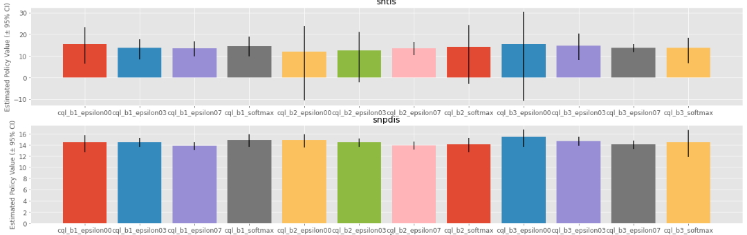
Policy Value Estimated by OPE Estimators
Users can implement their own OPE estimators by following the interface of BaseOffPolicyEstimator.
In addition, OffPolicyEvaluation summarizes and compares the estimation results of various OPE estimators.
See also
Cumulative Distribution OPE#
while the basic OPE is beneficial for estimating the average policy performance, we are often also interested in the performance distribution of the evaluation policy and risk-sensitive performance metrics including conditional value at risk (CVaR). Cumulative distribution OPE enables estimating the following cumulative distribution function and risk functions derived by CDF.
The following shows the example of estimating the cumulative distribution function of the trajectory-wise rewards and its statistics using Cumulative Distribution OPE estimators [8, 9, 10].
# import SCOPE-RL modules
from scope_rl.ope import CumulativeDistributionOPE
from scope_rl.ope.discrete import CumulativeDistributionDM as CD_DM
from scope_rl.ope.discrete import CumulativeDistributionTIS as CD_IS
from scope_rl.ope.discrete import CumulativeDistributionTDR as CD_DR
from scope_rl.ope.discrete import CumulativeDistributionSNTIS as CD_SNIS
from scope_rl.ope.discrete import CumulativeDistributionSNTDR as CD_SNDR

# (4) Evaluate the learned policy using the cumulative distribution function (in an offline manner)
# we compare ddqn, cql, and random policy defined in the previous section (i.e., (3) of basic OPE procedure)
# initialize the OPE class
cd_ope = CumulativeDistributionOPE(
    logged_dataset=test_logged_dataset,
    ope_estimators=[
    CD_DM(estimator_name="cdf_dm"),
    CD_IS(estimator_name="cdf_is"),
    CD_DR(estimator_name="cdf_dr"),
    CD_SNIS(estimator_name="cdf_snis"),
    CD_SNDR(estimator_name="cdf_sndr"),
    ],
)
# estimate variance
variance_dict = cd_ope.estimate_variance(input_dict)
# estimate CVaR
cvar_dict = cd_ope.estimate_conditional_value_at_risk(input_dict, alphas=0.3)
# estimate and visualize cumulative distribution function
cd_ope.visualize_cumulative_distribution_function(input_dict, n_cols=4)
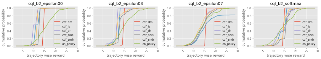
Cumulative Distribution Function Estimated by OPE Estimators
Users can implement their own OPE estimators by following the interface of BaseCumulativeDistributionOPEEstimator.
In addition, CumulativeDistributionOPE summarizes and compares the estimation results of various OPE estimators.
Off-Policy Selection and Evaluation of OPE/OPS#
Finally, we provide the code to conduct OPS, which selects the “best” performing policies among several candidates.
# import SCOPE-RL modules
from scope_rl.ope import OffPolicySelection

# (5) Conduct Off-Policy Selection
# Initialize the OPS class
ops = OffPolicySelection(
    ope=ope,
    cumulative_distribution_ope=cd_ope,
)
# rank candidate policies by policy value estimated by (basic) OPE
ranking_dict = ops.select_by_policy_value(input_dict)
# rank candidate policies by policy value estimated by cumulative distribution OPE
ranking_dict_ = ops.select_by_policy_value_via_cumulative_distribution_ope(input_dict)

# (6) Evaluate OPS/OPE results
# rank candidate policies by estimated lower quartile and evaluate the selection results
ranking_df, metric_df = ops.select_by_lower_quartile(
    input_dict,
    alpha=0.3,
    return_metrics=True,
    return_by_dataframe=True,
)
# visualize the top k deployment result
# compared estimators are also easily specified
ops.visualize_topk_policy_value_selected_by_standard_ope(
    input_dict=input_dict,
    compared_estimators=["cdf_dm", "cdf_is", "cdf_dr", "cdf_snis", "cdf_sndr"],
    safety_criteria=1.0,
)
# visualize the OPS results with the ground-truth metrics
ops.visualize_variance_for_validation(
    input_dict,
    share_axes=True,
)
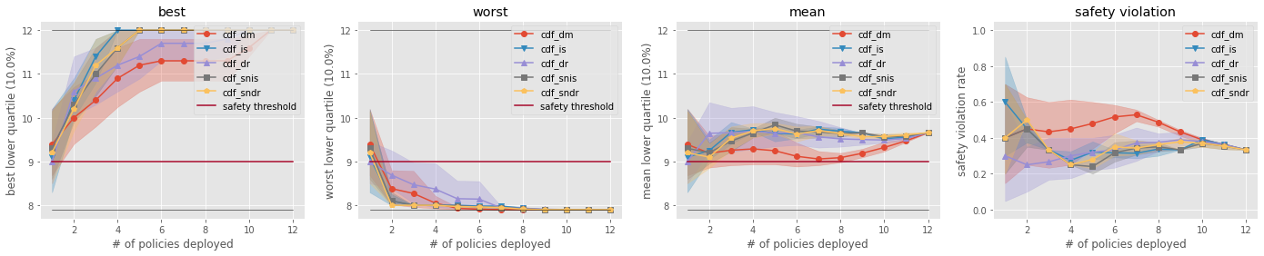
Comparison of the Top-k Statistics of 10% Lower Quartile of Policy Value
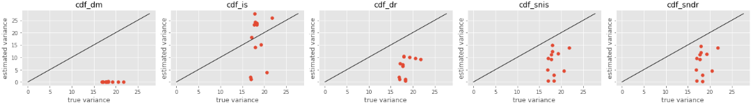
Validation of Estimated and Ground-truth Variance of Policy Value