Visualization Tools#

SCOPE-RL also provides user-friendly tools to visually compare and understand the performance of OPE methods. Specifically, the following figures are all available by calling only one function from either OffPolicyEvaluation, CumulativeDistributionOPE, or OffPolicySelection as follows.

# initialize the OPE class
ope = OPE(
    logged_dataset=logged_dataset,
    ope_estimators=[DM(), TIS(), PDIS(), DR()],
)
# conduct OPE and visualize the result
# by calling only one function!
ope.visualize_off_policy_estimates(
    input_dict,
    random_state=random_state,
    sharey=True,
)

Then, the above code produces the following visualization result.

Policy value estimated by (standard) OPE Estimators

Similarly, visualization tools are also available for cumulative distribution OPE (CD-OPE).

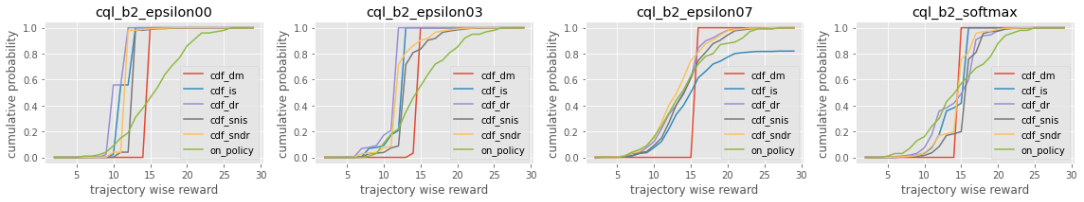
Cumulative distribution function estimated by CD-OPE Estimators

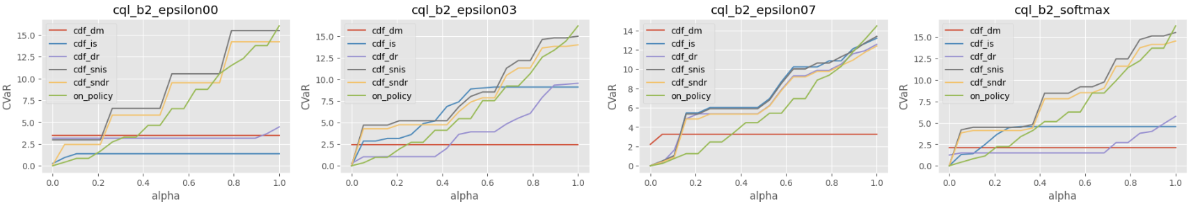
Conditional value at risk (CVaR) estimated by CD-OPE Estimators

Policy value and its confidence interval derived by variance estimated by CD-OPE Estimators

Interquartile range estimated by CD-OPE Estimators

Moreover, the evaluation of OPE/OPS can also be done by visualizing the top-\(k\) Risk-Return Tradeoff (RRT) metrics. Note that the following figures are applicable to all the point-wise performance estimates including expected policy value, variance, CVaR, and lower quartile.

Example of evaluating OPE/OPS methods with top-\(k\) RRT metrics

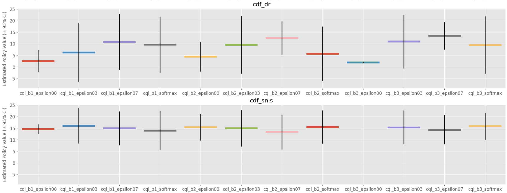
Furthermore, when conducting OPE on multiple logged datasets collected by various behavior policies, SCOPE-RL also enables a discussion on how the quality of the dataset may affect the performance of OPE.

First, the following three figures are applicable to the point-wise estimate of expected policy value, variance, CVaR, and lower quartile. In the following example, we can learn that OPE results can be particularly unstable when using “ddqn_epsilon_0.1” as the behavior policy, which is more deterministic than other behavior policies.

Policy value estimated on the multiple datasets collected by various behavior policies (box)

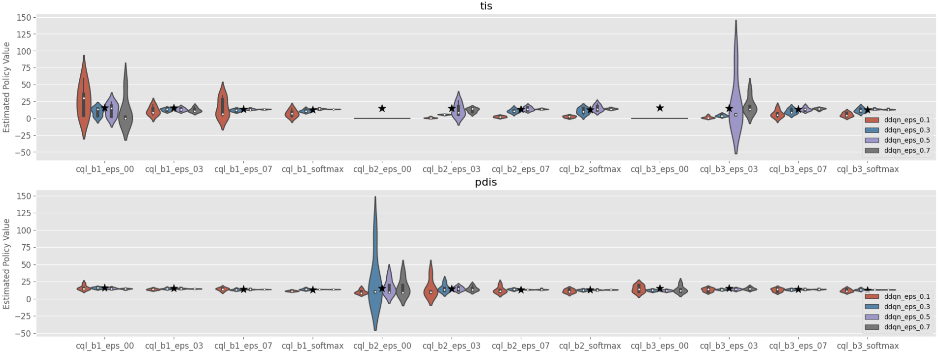
Policy value estimated on the multiple datasets collected by various behavior policies (violin)

Policy value estimated on the multiple datasets collected by various behavior policies (scatter)

Next, we demonstrate the example of comparing cumulative distribution function estimated on multiple logged datasets collected by various behavior policies. In the figure, we observe that the cumulative distribution OPE results do not change greatly across various behavior policies.

Cumulative distribution function estimated on the multiple datasets collected by various behavior policies

Finally, we compare the true policy value (x-axis) and estimated policy value (y-axis) in the following figure. For TIS, PDIS, and DR, the result suggests that the variance of OPE estimation becomes particularly large when using a near-deterministic behavior policy named “sac_sigma_0.5”. On the other hand, for SNTIS and SNPDIS, we found that the choice of behavior policy can heavily affect the estimation result of OPE – OPE results are almost the same across various evaluation policies in the bottom left figures. This kind of visualization is again available for all point-wise estimates including expected policy value, variance, CVaR, and lower quartile.

Validation results of the policy value estimation on multiple logged datasets collected by various behavior policies